SVD(Singular Value Decomposition) and PCA(Principle Component Analysis) in Real-life Applications
Connections between SVD and PCA & Real-life Applications.


- Mathematical Theory of SVD
- Mathematical Theory of PCA
- Connections between SVD and PCA
- Real-life Applications of SVD and PCA
- Summary
- References
It is usually necessary to observe the data with multiple variables in many research and application fields, and how to analyze and find rules to construct appropriate models via the large amount of data is always the main topic. Multivariate large datasets undoubtedly provide rich information for research and application, but inversely, they will increase the workload of data collection to some extent. Furthermore, there may exist correlations among many variables in many cases, which will definitely increase the complexity of data analysis. If variables are analyzed separately, the analysis is often isolated and the information behind the data cannot be fully utilized. Therefore, the blind reduction of indicators will lose a lot of useful information, resulting in wrong conclusions. But the realistic problem is that huge amount of data cannot be stored and analysed in a reasonable and understandable way. We must find the balance between data utilization and dimension reduction.
We can have an intuitive example about the disaster gotten from high dimensional data. Different from text information, image information occupies a large capacity so that its storage and transmission will be greatly limited. Assume there is a still color image and its size is $1200\times1200$, which means it's $1200$ pixels long and $1200$ pixels wide and there are $1440000$ pixels on the screen. A pixel of a still color image needs three memory cells, so the single image needs $3*1440000=4320000=4218.75$KB disk storage space. If the color image is transmitted at $24$ frames per second, the amount of data per second is $24*4218.75$KB$\approx99$MB, then a $640$MB CD-ROM can only store about $6.5$ seconds of original data. With the present technology, it is difficult to meet the storage and transmission needs of the original digital image. We all know that image processing is an important task in the field of machine learning, so it is inevitable that we have to do something on the target images to compress the images and extract important features.
Therefore, it is necessary to find a reasonable method to reduce the loss of information contained in the original indicators while reducing the indicators to be analyzed, so as to achieve the purpose of comprehensive analysis of the collected data. Since there is a certain correlation between the variables, we can consider changing the closely related variables into as few new variables as possible, so that these new variables are uncorrelated, then we can use less comprehensive indicators to represent the various kinds of information in each variable. Dimension reduction is a preprocessing method for high dimensional feature data. Dimension reduction is to preserve some of the most important features of high-dimensional data, remove noise and unimportant features, so as to improve the speed of data processing. In the actual production and application, dimension reduction can save us a lot of time and cost in a certain range of information loss. Dimension reduction has become a widely used data preprocessing method and the kind of reduction has several strong points:
- Make the dataset feasible to explore and utilize
- Decrease the number of feartures (only reserve the most important features)
- Make sure the independence between features
- Decrease the cost of algorithms
- Make the results understandable
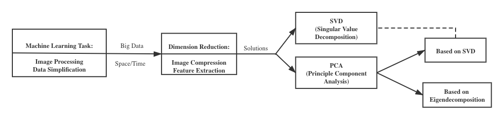
So how to reduce dimensions like image compressing and features extraction is worth deep thinking. Thanks to the SVD(singular value decomposition), which is a descent algebraic transformation, we can use the optimal matrix decompostion to do the image compression. Meanwhile, there is another similar method called PCA(principle component analysis) which is also used the matrix transformation and decomposition. The two methods have some connections and differences, they also have their own advantages. I want to introduce the mathematical conceptions behind SVD and PCA, explain the connections and differences between the two methods and compare the two methods via same tasks.
We have the traget matrix $A$ which is an n $\times$ n real matrix and an $n$-dimension vector $x$. We first review the definitions of eigenvalues and eigenvectors: $Ax = \lambda x$. In this formula, $\lambda$ is an eigenvalue of matrix $A$, and $x$ is the eigenvector corresponding to the eigenvalue $\lambda$.
After we know the according eigenvalues and eigenvectors, we can do eigenvalue decomposition to the matrix $A$. Now we have n eigenvalues of matrix $A$: $\lambda_1 \leq \lambda_2 \leq \cdots \leq \lambda_n$ and the according eigenvectors {$v_1,v_2,\cdots,v_n$}, if the $n$ eigenvectors are linearly independent, then the matrix can be eigen decomposed as $A = V\Lambda V^{-1}$. $V$ is an n$\times$n matrix composed of the $n$ eigenvectors and $\Lambda$ is the n$\times$n matrix with $n$ eigenvalues on its main diagonal. Generaly, we will normalize the $n$ eigenvectors in matrix $V$, namely satisefying $||v_i||_2 = 1$, or $v_i^T v_i = 1$. At this time, the eigenvectors of $V$ are the standard orthogonal bases, satisefying $V^TV=I$, namely $V^T = V^{-1}$. Then we can rewrite the eigenvalue decomposition of matrix $A$: $A = V\Lambda V^T$.
To clarify one important point of eigenvalue decomposition: the matrix $A$ must be a square matrix. So another question comes up: if the matrix $A$ is not a square matrix which means that the numbers of columns and rows are not the same, can we decompose the matrix $A$? The answer is definitely yes, and it just introduces the main topic SVD(singular value decomposition).
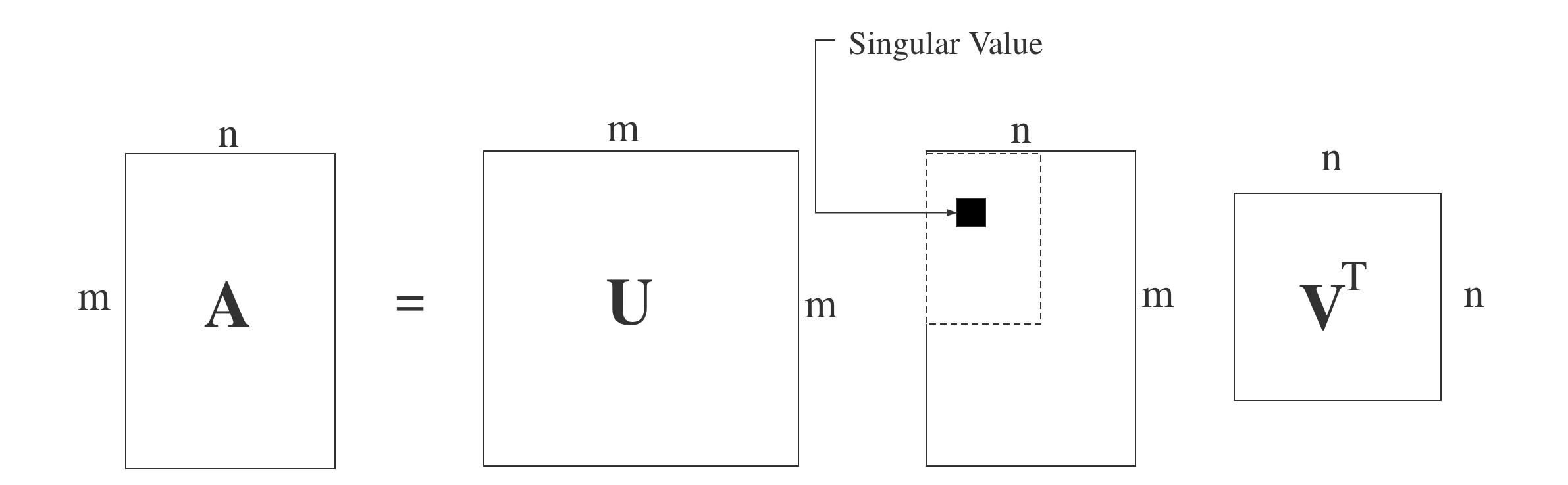
SVD is another method to decompose a matrix. Different from the eigenvalue decomposition, SVD does not require the decomposed matrix to be the square one. Assume we have an m$\times$n target matrix A, then we can create an m$\times$m matrix $U$, an n$\times$n matrix $V$ and an m$\times$n matrix $\Sigma$ with singular values on the main diagonal. Using these created matrices, we can define SVD of matrix $A$ as: $A = U\Sigma V^T$. The matrice $U$ and $V$ satisefy $U^TU=I$ and $V^TV=I$. The following image can express the decomposition process clearly.
We all know that the matrix A here is not a square matrix, so we can do the matrix multiplication of $A^T$(the transpose of A) and A. Then we can get an n x n matrix $A^TA$. Since the new created matrix $A^TA$ is a square one, we can do the eigen decomposition to them. Assume the target matrix is $A^TA$ now, then the following formula can represent the process: $(A^TA)v_i = \lambda_iv_i$. According the formula, we can get the n eigenvalues and the n according eigenvectors $\boldsymbol{v}$. We can get the matrix $V$ using all eigenvectors of $A^TA$, the matrix $V$ is just the same $V$ in the formula of SVD. Generally, we call each eigenvector in matrix $V$ the right singular vector of $A$.
Then we will do all same steps to $AA^T$ as to $A^TA$. Obviously we can get $(AA^T)v_i = \lambda_iu_i$. Similarly, we call each eigenvector in matrix $U$ the left singular vector of $A$.
Now we have solved matrices $U$ and $V$, the only problem is how to calculate the singular matrix $\Sigma$. We know that $\Sigma$ only has the singular values on the main diagonal and all other positions with value 0. So we only need to solve each singular value $\sigma_i$. We can use the original SVD formula $A = U\Sigma V^T$ and use matrix multiplication to multiply matrix $V$ in both sides of the equation: $$ A = U\Sigma V^T \Rightarrow AV = U\Sigma V^TV \Rightarrow AV = U\Sigma \Rightarrow Av_i = \sigma_iu_i\Rightarrow \sigma_i = Av_i/u_i $$
We can also verify that the eigenvectors of $A^TA$ and $AA^T$ make up the matrix $V$ and matrix $U$ in SVD using the knowledge that $U^TU=I$, $V^TV=I$ and $\Sigma^T\Sigma = \Sigma^2$: $$ A = U\Sigma V^T \Rightarrow A^T = V\Sigma^T U^T \Rightarrow \begin{cases} A^TA = V\Sigma^T U^T U \Sigma V^T = V\Sigma^2V^T \cr AA^T = U \Sigma V^T V\Sigma^T U^T = U\Sigma^2U^T \end{cases} $$ Furthermore, we can get that the eigenvectors matrix equals to the square of singular value vectors matrix which means we can know the relationship between the eigenvalues and singular values: $\sigma_i = \sqrt{\lambda_i}$.
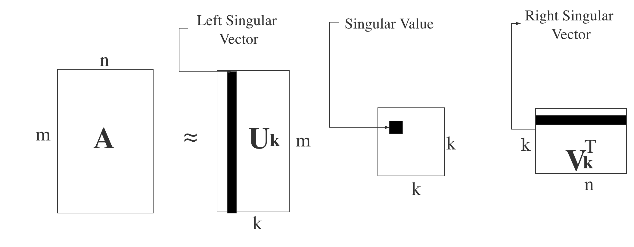
Similar to the eigenvalues in eigen decomposition, the singular values arrange from large to small in the singular values matrix, also the values decrease fast. That is to say, the sum of first $20$% or even $1$% of the whole singular values will account for more than $99$% of the sum of all singular values generally. In another word, the useful property of SVD is that we can use the largest $k$ singular values and the corresponding singular vectors to approximately represent the target matrix. We use $k$ colums in matrix $U$ and $k$ rows in matrix $V^T$. The whole process can be represented as the following formula: $$ A_{mxn} = U_{mxm}\Sigma_{mxn}V^T_{nxn}\approx U_{mxk}\Sigma_{kxk}V^T_{kxn} $$ Since $k$ is much smaller than $n$, the large target matrix $A$ can be represented by three much smaller matrices $U_{mxk}$, $\Sigma_{kxk}$, $V^T_{kxn}$. We can use a diagram to represent the process.
The meaning of PCA(principle component analysis) is to find the most inportant part of data to substitute the raw data. PCA is one of the most important dimension reduction methods. In detail, assume we have an $n$ dimension dataset with $m$ data $(x_1,x_2,\cdots,x_m)$. We want to reduce the dimensions of this data from $n$ dimensions to $k$ dimensions, and hope the $k$ dimensions data can best represent the raw data. The loss cannot be inevitable during the dimension reduction process, so we want to minimaize the loss.
We can see a very easy condition where $n$=$2$ and $k$=$1$. That is to say, the task is to reduce the dimensions of the data from $2$ to $1$. The data are shown as below.
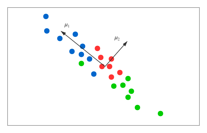
According to the diagram above, we want to find one direction to represent the $2$-dimension data. We have two vectors listed in the diagram $\mu_1$ and $\mu_2$. Obviously, we will choose $\mu_1$. There are two main reasons. One is that the projections of the data on the line of $\mu_1$ direction will be best separate, the other is that the distances from the sample data to the line are enough small. If we want to make the $k$ from $1$ dimension to any dimensions, the criteria have the same thoughts: the projections of sample data on the hyperplane must be separatable enough and the distances between sample data and the hyperplane must be small enough.
Assume we have $m$ $n$-dimension de-meaned data $(x_1, x_2, \cdots, x_m)$, which means that the sum of the $m$ data is $0$. All $m$ data satisefy that $\sum_{i=1}^{m}{x_i}$=$0$. Also, we can assume that the new coordinate system using the bases after the projection transformation will be {$\boldsymbol {w_1, w_2, \cdots, w_n}$}, and $\boldsymbol w$ is the orthonormal basis. What we want to do in PCA is to reduce the dimensions from $n$ to $k$, which means that we need to drop some useless coordinates and create a new coordinate system {$\boldsymbol {w_1, w_2, \cdots, w_k}$}. Then one of the sample data $x_i$ will have the expression for its projection in this $k$-dimension coordinate system: $p_i$ = $(p_{i1}, p_{i2}, \cdots, p_{ik})^T$, and $p_{ij}$=$w_j^T x_i$ which means that the it is the coordinate of $x_i$ in the $j$th dimension of the original $n$-dimension coordinate system, namely $w_j$.
For any sample data $x_i$, it has the projection $W^Tx_i$ and the projection variance $x_iWW^Tx_i$. We want to maximize the sum of the projection variance of all sample data, so we will maximize the trace of $\sum_{i=1}^{m}{W^Tx_ix_i^TW}$, the following formula represents the whole thing:
Objective function: ${argmax}$ $tr(W^TXX^TW)$
Constarint function: $ W^TW = I$
To solve the above optimization problem, we can introduce the Lagrange multiplier $\lambda$ to get the new Lagrange function: $$ L(W) = tr(W^TXX^TW + \lambda(W^TW-I)) $$ Then we can do the derivative for argument $W$ and we can get that: $$ XX^TW + \lambda W = 0 \Rightarrow XX^TW = -\lambda W $$
Interestingly, we can find that the expression is very similar to the eigenvalue decomposition, so we can do some conclusions about the matrix $XX^T$ and the meaning of $-\lambda$. We can say that $W$ is the matrix which consists of the $k$ eigenvectors of matrix $XX^T$ and $-\lambda$ is just the eigenvalue matrix with eigenvalues on the diagonal and $0$ on other positions. Whenever we want to do the dimension reduction, we just need to find the corresponding eigenvectors of the $k$ biggest eigenvalues. The $k$ eigenvectors just construct the needed matrix $W$.
If you want to learn more about the process of PCA, please refer to
wikipedia:https://en.wikipedia.org/wiki/Principal_component_analysis
We want to give an easy example that can represent the process of PCA clearly and understandably.
Assume we have a matrix $X$ = $\left\lgroup\begin{matrix}-1 & -1 & 0 & 2 & 0 \cr -2 & 0 & 0 & 1 & 1\end{matrix}\right\rgroup$, we want to use PCA to make the $2$-dimension data to $1$-dimension.
X = [-1 -1 0 2 0; -2 0 0 1 1]
- Make sure the target matrix is de-meaned.
println(mean(X[1,:]))
println(mean(X[2,:]))
We can find that the mean value of each line of the matrix $X$ is $0$, so we do not need to do any change.
- Calculate the covariance matrix.
The covariance matrix is $\frac{1}{n}XX^T$. (the use of $\frac{1}{n}$ or $\frac{1}{n-1}$ does not have too much influence)
cXXᵀ = 1/length(X[1,:]) * X * X'
The whole calculation of the covariance process is $$ cXX^T = \frac{1}{5} \left\lgroup\begin{matrix}-1 & -1 & 0 & 2 & 0 \cr -2 & -0 & 0 & 1 & 1\end{matrix}\right\rgroup \left\lgroup\begin{matrix}-1 & -2 \cr -1 & 0 \cr 0 & 0 \cr 2 & 1 \cr 0 & 1 \end{matrix}\right\rgroup = \left\lgroup\begin{matrix}1.2 & 0.8 \cr 0.8 & 1.2\end{matrix}\right\rgroup $$
- Calculate the eigenvalues and eigenvectors of the covariance matrix.
eigvals(cXXᵀ)
P = -eigvecs(cXXᵀ)
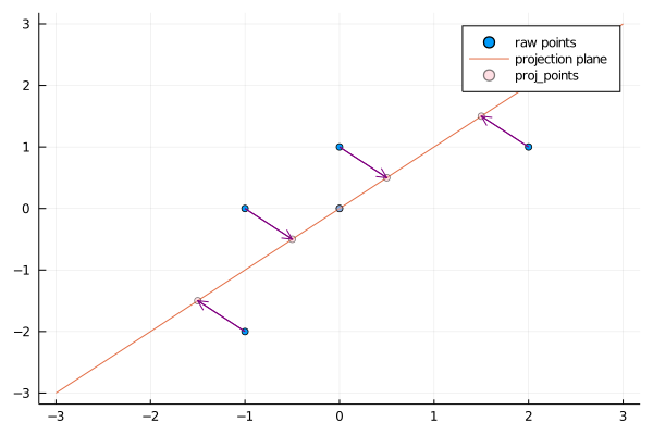
By calculation, we can get that the eigenvalues are $\lambda_1=2$ and $\lambda_2=0.4$. The corrsponding eigenvectors are $v_1$ = $\left\lgroup\begin{matrix}\frac{1}{\sqrt 2} \cr \frac{1}{\sqrt 2}\end{matrix}\right\rgroup$ and $v_2$ = $\left\lgroup\begin{matrix}-\frac{1}{\sqrt 2} \cr \frac{1}{\sqrt 2}\end{matrix}\right\rgroup$, then we can get the matrix $P$ = $\left\lgroup\begin{matrix}\frac{1}{\sqrt 2} \frac{1}{\sqrt 2} \cr -\frac{1}{\sqrt 2} \frac{1}{\sqrt 2}\end{matrix}\right\rgroup$.
- Get the dimension reduction reuslt
We need to get the $1$-dimention result, so we only get the eigenvector corresponding to the largest eigenvalue.
We can use julia to get the same result, and also we can have a very clear diagram to see the whole process.
Generally speaking, if we want to use PCA to reduce dimensions, we need to find the $k$ eigenvectors corresponding to the $k$ largest eigenvalues of the covariance matrix $\frac{1}{n}X^TT$. Then we can use the projection matrix consisting of the $k$ eigenvectors as the projection hyperplane. From the process, we can know that it is inevitable that we always need to get the result of the covariance matrix $\frac{1}{n}X^TX$. But when the features of the sample data are very large, the calculation process will be both time comsuming and space consuming.
We can also use SVD to get the projection matrix using the $k$ eigenvectors. But the reason why I want to mention about the advantages of SVD is that some algorithms of SVD can still get the result of right sigular matrix $V$ without calculating the covariance matrix $\frac{1}{n}X^TX$. That is to say, our PCA algorithms do not need to do the eigenvalue decomposition, instead, we can let SVD to complete this. This method is very effective and efficient when the sample data are very large.
In this part, we want to verify two conclusions:
- There are square relationships between singular values and eigen values
- The results of singular value decomposition and eigenvalue decomposition of covariance matrix are consistent
Firstly, we will verify the first conclusion. We want to get some interesting relationships about covariance matrix $\frac{1}{n}X^TX$, but we only focus on parts of the matrix $X^TX$ for convenience. According to the definition of sigular value decompsition: $X = U\Sigma V^T$, we can get that $$X^TX = V\Sigma U^TU\Sigma V^T = V\Sigma^2V^T = V\Sigma^2V^{-1}.$$ And we know that $X^TX$ is a symmetric positive semidefinite matrix, so it can be eigenvalue decompsed as $$ X^TX = V\Lambda V^{-1}. $$ We can find that the two formula are consistent. And when the order of eigenvalues is assigned, we can easily find that $$\Lambda = \Sigma^2.$$
Given an SVD of matrix $X$($X = U\Sigma V^T$), we know that
- The columns of $V$(right singular vectors) are eigenvectors of $X^TX$;
- The columns of $U$(left singular vectors) are eigenvectors of $XX^T$.
If you do not know this, you can refer to https://en.wikipedia.org/wiki/Singular_value_decomposition#Relation_to_eigenvalue_decomposition
Bearing the above two in the mind, we can make SVD on $X^TX$. Given that $X^TX = U_2\Sigma_2V_2^T$, we can know that $U_2$ is just the eigenvectors of $X^TXX^TX$(we can write the new matrix as $(X^TX)(X^TX)^T$).Then we can get that: $$ X^TXX^TX = U_2\Sigma_2V_2^T(U_2\Sigma_2V_2^T)^T = U_2\Sigma_2^2U_2^T $$ And according to eigenvalue decompsition, we can get that $X^TX = V_2\Lambda_2V_2^{-1}$, so for the new matrix, we can get that: $$ X^TXX^TX = V_2\Lambda_2^2V_2^{-1} $$ Easily, we can find that $U_2=V_2$ and $\Sigma_2^2 = \Lambda_2^2$.
Based on the verification that the SVD has the same result as eigenvalue decompsition of convariance matrix, we can do PCA based on SVD.
The whole implementation process is not difficult.
Input: dataset $X$ = {$x_1$, $x_2$, $\cdots$, $x_n$}
Target: Reduce the dimensions from $n$ to $k$
Process:
- De-meaned
- Calculate the covariance matrix
- Calculate the eigenvectors and eigenvalues based on SVD
- Sort eigenvalues from large to small and choose the first $k$ largest eigenvalues and corresponding eigenvectors.
- Make the dataset into the new $k$ dimensions space via linear transfromation
There is another interesting aspect deserves exploration. We can explore meanings of left singular matrix $U$ and right singular matrix $V$. $$ X^l_{k\times n} = U^T_{k\times m}X_{m\times n} $$ We can easily find that the new matrix $X^l$ condenses the rows from $m$ to $k$ compared to the raw matrix $X$. So we can get the conclusion that the left singular matrix can condense the rows number. For the matrix $V$, we can assume the same sample data matrix which is m$\times$n. Then we find the right singular matrix $V$ using the $k$ eigenvectors of matrix $\frac{1}{n}XX^T$ from SVD, then we can a new matrix $X^r$: $$ X^r_{m\times k} = X_{m\times n}V^T_{n\times k} $$ In this case, the right singular matrix can reduce dimensions for columns. When we use SVD to decompose covariance matrix to realize PCA (PCA based on SVD), and we can get PCA dimension reduction in two directions (row and column).
Then we want to use a diagram to illustrate the connections between SVD and PCA.
In this part, We want to show applications of the SVD and PCA in real life. The applications will include:
- a mathematical example which calculates a simple matrix using different methods
- iris dataset examples which use first three features for plotting a 3-d image and first two features for comparison
- vivid image processing examples.
We hope you can have fun in this part.
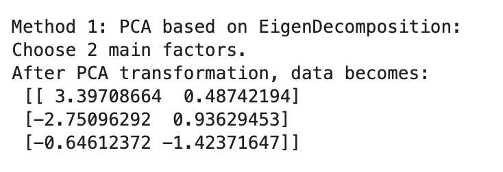
The raw matrix is $\left\lgroup\begin{matrix}-2 & -1 & 0 & 2 & 1 \cr 2 & 2 & 0 & -1 & -1 \cr 2 & 0 & 1 & 1 & 0 \end{matrix}\right\rgroup$. Then we will do the basic PCA(based on eigenvalue decomposition) to this data and choose two most important features, and we can get the result reduced matrix. In the process, we can easily calculate the covariance matrix cov_Mat, then we just use the basic algorithm of PCA which is using the eigen decomposition to get the eigenvalues $\Lambda$ and eigenvectors $V$. We will rearrange the eigenvectors and eigenvalues. For eigenvalues, we will choose eigenvalues by component or rate, then we can get the corresponding eigenvectors. Lastly, we can do some data transfromation to get the output data. And we can see the results using this PCA based on eigendecomposition:
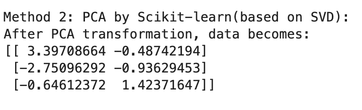
Then we want to do PCA based on SVD on the same raw matrix. Thanks to Scikit-learn, we can just use the PCA function and choose the component=$2$ and then use fit! to fit the pca model. Lastly, we can get the output data.
The last method is using SVD directly. We just use the svd function to get the right sigular vector matrix $U$, the left sigular vector matrix $V$ and the singular value matrix $\Sigma$. Then we can choose how many factors we need to use in this decomposition. Lastly, we can transform data to get the output result.
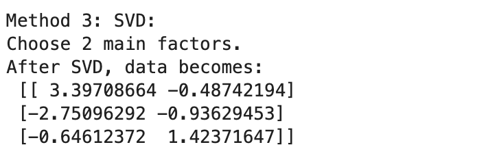
We can see that the SVD and PCA methods generally have the same result for simple data, the three methods are all feasible.
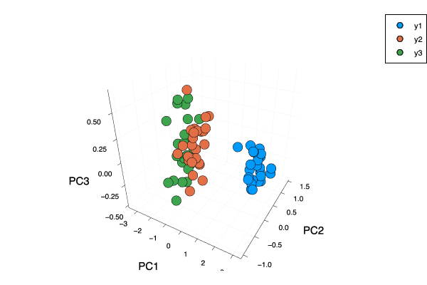
In this part, We will use the iris dataset as examples. We use the same dataset to do two things. The first is that we can see the $3$-dimension result(instead of just on a plane) vividly via choosing three features. The second is that we want to do the normal things: choose two features of the iris dataset and use different methods to compare results.
Firstly, I want to use the MultivariateStats package in julia which contains PCA function to do the dimension reduction operation. I choose the first $3$ principal components and then use scatter and plot functions in Plots package to show a $3$-dimension diagram.
The PCA function in MultivariateStats package has two core algorithms: pcacov and pcasvd. From the names, we can see that one algorithm uses the eigendecomposition of covariance matrix and the other one just uses SVD. The two algorithms have different parameters, the PCA function will call different algorithms based on different parameters. pcacov function has param C for covariance matrix and param mean for the mean vector of original samples. pcasvd function has param Z for centralized samples and param mean for the mean vector of original samples. For detailed information about this package, you can refer to: https://multivariatestatsjl.readthedocs.io/en/latest/pca.html .
And we can see the $3$-dimension plot with first three principle features.
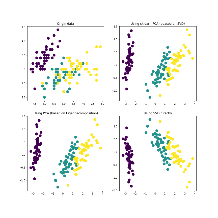
Then we want to choose the first two principle features and use PCA(based on SVD), PCA(based on eigenvalue decomposition) and direct SVD methods. We can see the four plots vividly.
To make the algorithms diverse, we use the PCA based on SVD so that we can directly call the PCA function in sklearn.decomposition. For the PCA based on eigenvalue decomposition, we need to caculate the covariance matrix. For direct SVD, we can use svd function to get the needed matrices $U$, $\Sigma$ and $V$.
This part is very interesting. We first use the direct SVD method to an .png image file, and we choose different feature numbers to see the results of image compression. Then as normal, we will use SVD and PCA to one image and see the results of different methods.
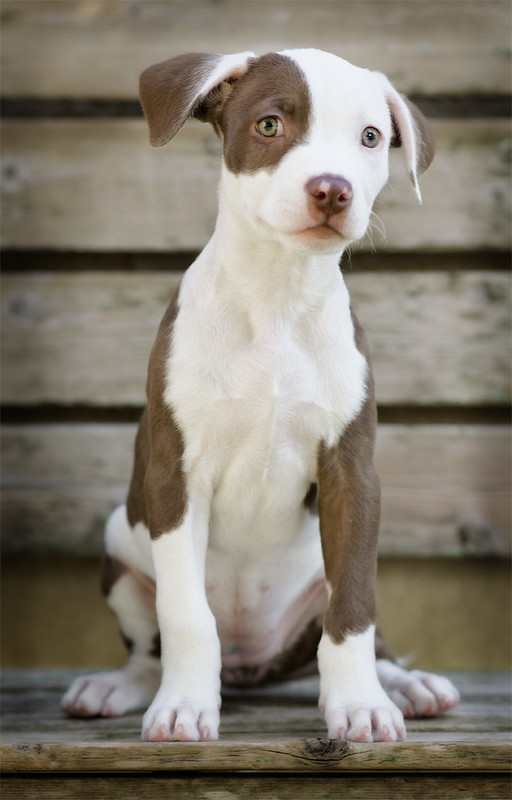
The following is an image with $800\times512$ pixels. We want to know how to work with color channels to explore image compression using the SVD. We can see that the details including the colors, outlines and so on are very clear in this raw image.
We know that the raw image above is $800\times512$, which means that the raw image has at most $512$ sigular values. Then we want to choose $10$, $50$, $100$ singular values respectively and get the according results compared with the raw image. We use the map function in julia language to choose different sigular values and use mosaicview function to show the results including the raw image in the first place. The result is shown as below:
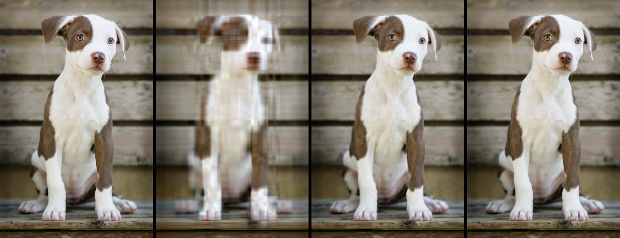
It is not difficult to find that the compressed image is very fuzzy when choosing only $10$ singular values. The outlines and the patterns of the lovely dog cannot be dealt with clearly, which means that the first $10$ singular values cannot closely represent the whole information of the raw image. When we choose $50$ singular images, we can see that the ouline of the dog is only a little fuzzy. And when we choose $100$ singular values, we find it is very close to the raw image. That is to say, we can only use $100$ singular values instead of $512$ total to represent to dog image which means that less space to store the needed information and less time to deal with the related information. Without doubt, SVD is very useful and successful in image compression.
Then we will do the same step as the previous examples. We want to compare the results of SVD and PCA to the same image. The cat.png image file is a cat with a mask, it is $1200\times1200$ pixels. We use direct SVD method and PCA based on eigenvalue decompostion method to compress the raw image. To make the problem simple, we transfer the RGB image to Gray image.

We can see that the two images on the first row are the raw image and the corresponding gray image. Then we just get the matrices $U$, $V$ and $\Sigma$ via the embedded function svd(). When it comes to PCA methods, we use the covariance matrix and calculate the eigenvalues and eigenvectors. We can see that both compressed images represetnt the raw gray image very well.
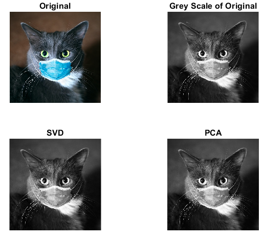
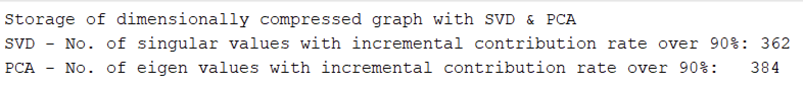
To explore deeper about the difference of SVD and PCA, we write another function to calculate how many corresponding values(singular values in SVD, eigenvalues in PCA) can represent $90$% cumulative contribution rate for the raw gray image in different methods. We need $384$ eigenvalues in PCA while we only need $362$ singular values in SVD. So it is not difficult to summarize that the SVD method will do better on image compression on the same level.
This blog clarifies the methematical theories behind SVD and PCA using some formula. We just give some simple derivation processes like how to caculate the singular vectors and singlar values in SVD and how to get the eigenvalues and eigenvectors of covariance matrix in PCA. If you want to explore deeper and wider, you can click on the links, I think they are very useful.
A very important topic in this blog is that there are two main algorithms in PCA. One is PCA based on eigenvalue decomposition which uses covariance matrix and the other is PCA based on SVD which uses singular values and singular vectors. Because the basic PCA based on eigenvalue decomposition cannot do as well as the PCA based on SVD in general, so some embedded PCA functions like PCA in MultivariateStats and PCA in sklearn.decomposition both use PCA based on SVD which is verified more effective and efficient.
The most interesting part of this blog is the vivid examples. We illustrate examples using simple matrices, iris dataset and some images. We hope you can find the connections and differences between different methods. Hope you can understand easily with the help of these diagrams.
[1] https://en.wikipedia.org/wiki/Singular_value_decomposition#Relation_to_eigenvalue_decomposition
[2] https://en.wikipedia.org/wiki/Principal_component_analysis
[3] https://multivariatestatsjl.readthedocs.io/en/latest/pca.html
[4] https://juliaimages.org/latest/democards/examples/color_channels/color_separations_svd/